LTE and RADEX Analysis
| Contents |
Utility of the LTE and RADEX analysis tool
CASSIS can model astronomical spectra using plugged-in models. Presently a Local Thermodynamic Equilibrium model (described here) and a statistical equilibrium radiative transfer code, RADEX, (described here), using the Leiden Atomic and Molecular Database (described here), are available. RADEX is a one-dimensional non-LTE radiative transfer code, that uses the escape probability formulation assuming an isothermal and homogeneous medium without large-scale velocity fields. RADEX is comparable to the LVG method (see our LVG documentation) and provides a useful tool in rapidly analyzing a large set of observational data providing constraints on physical conditions, such as density and kinetic temperature.
How does it work?
Click on the third menu, Modules, and choose LTE + RADEX.
Alternatively, click on the icon  .
In both cases, a pop-up window opens:
.
In both cases, a pop-up window opens:
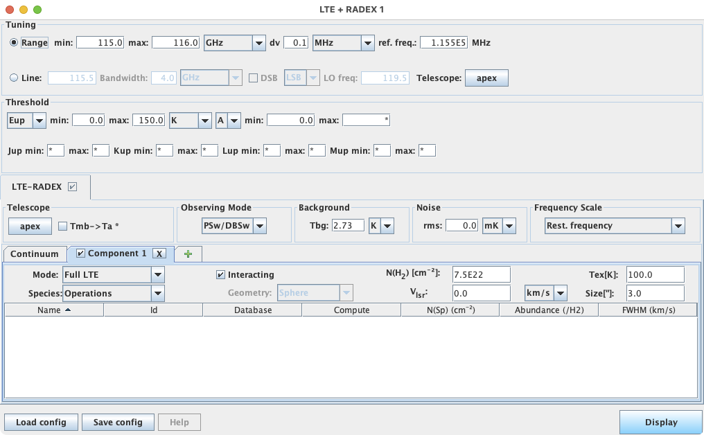
If you want to model a source, you need to specify the following parameters:
- Tuning panel:
- If you want a specific frequency range, select the Range [GHz] button and enter the minimum and maximum frequencies in GHz.
- If you want to center on a specific line, select the Line [GHz] button and
enter the line frequency in GHz.
NOTE: make sure you hit 'enter' after typing the line frequency value, in order to automatically update the frequency of the local oscillator (LO freq. [GHz] field), depending on the telescope you choose ; the later is done by clicking on the telescope name, which brings up a file browser.
If you want to model a spectrum in DSB mode, select the DSB button and choose in the pull-down menu the tuning band (LSB or USB) you want to use.
Additionally, you can set the bandwidth in GHz. - In both cases, you can set the spectral resolution
in the dv [MHz] box.
WARNING: a high spectral resolution combined with a broad spectral range yields a large number of points and hence increases the computing time and can lead to a memory overflow.
- Threshold panel:
You can select a (lower and/or upper) limit on the upper energy (Eup) of the lines you request, as well as the minimum Einstein coefficient (Aij min) and other quantum numbers. This will lower the calculation time. - Parameters panel:
- If tuning on a specific line, the telescope is automatically set to be the same as in the "Tuning" panel.
If tuning over a frequency range, set the desired Telescope by clicking on the
telescope name, which brings up a file browser from which you can choose the desired telescope file.
If the telescope you want does not exist, you can add it simply by
duplicating one of the telescope files in
YOUR_CASSIS_DIRECTORY/delivery/telescope/ and
changing the parameters to match those of the desired telescope.
WARNING: Take care that you do not change the format of the file ! - By default, CASSIS computes the spectrum in Tmb; however, if you want the modeled spectrum in Ta units, select the Tmb->Ta conv box.
- If tuning on a specific line, the telescope is automatically set to be the same as in the "Tuning" panel.
If tuning over a frequency range, set the desired Telescope by clicking on the
telescope name, which brings up a file browser from which you can choose the desired telescope file.
If the telescope you want does not exist, you can add it simply by
duplicating one of the telescope files in
YOUR_CASSIS_DIRECTORY/delivery/telescope/ and
changing the parameters to match those of the desired telescope.
- In the Noise panel, you can add a white noise by modifying the rms in milli-Kelvin.
- The Frequency scale panel allows you to choose between "Rest frequency" or "Sky frequency of the 1st component" for your model.
- The last panel concerns the source parameters. You can model as many lines as you want.
Depending on the line parameters you defined, the modeled spectrum will be in absorption or in emission
(see this document for more details).
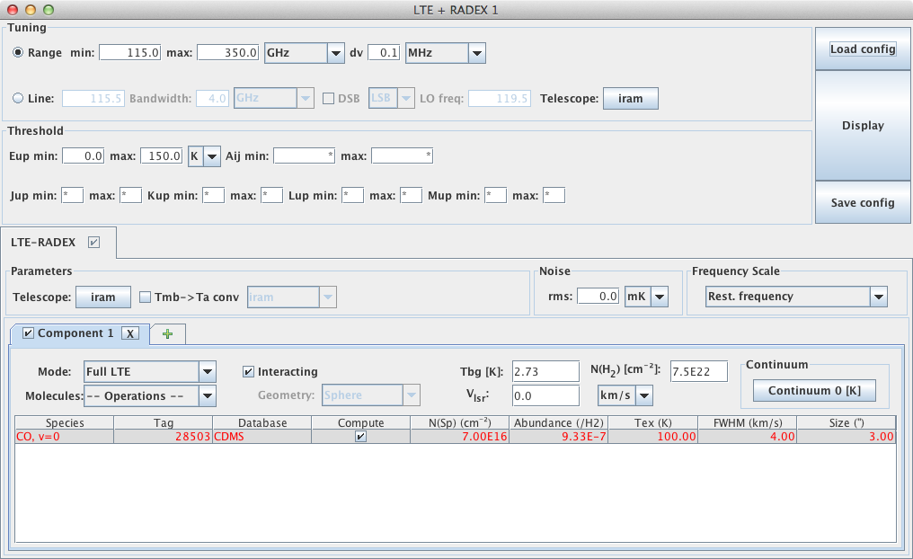
In the Mode pull-down menu, you can choose whether you want to model your lines in LTE only (Full LTE) or RADEX only (Full RADEX).
WARNING: choosing "Full RADEX" will only produce a model which includes lines that are tabulated in the LAMDA database.
On the right-hand side some parameters are listed:- Tbg [K] (RADEX only) : Rayleigh-Jeans equivalent temperature of the background radiation field, assumed to be of black body shape. Default is the cosmic microwave background.
- N(H2) [cm-2] : molecular hydrogen column density, needed in order to compute the overall abundance of the selected species;
- Vlsr [km/s] : velocity in the local standard of rest associated to each components.
- Continuum panel (for the 1st of all interacting component, and for all non-interacting
components): this allows you to simulate a spectrum with a continuum (in Kelvin) read from a file.
The file can be selected by clicking on the continuum box, which brings up a file browser.
Some continuum files are distributed with the software : "Continuum 0 [K]" (no continuum, default),
"Continuum 1 [K]" (1K continuum), "continuum-a", "continuum-b", "power0303" and "powerlaw" ; they are located in
"YOUR_CASSIS_DIRECTORY/delivery/continuum/".
You can create your own continuum file(s) and place them anywhere you like. These files must have the same format as those found in the above directory, that frequency in GHz in the first column and continuum in Kelvin in the second column, separated by one tabulation.
For example in order to model a 2.4 K continuum to the CO (1-0) line at 115.3 GHz with a tuning range between 101 and 139 GHz, duplicate one of the example files and replace the data by:
100.00 2.4
140.00 2.4
The numbers must be separated by 1 tabulation.
NOTE: When calculating a model, CASSIS uses a slightly larger range than the one specified in the "Tuning" panel (point 1) to avoid "cutting" a line profile in case it is close to one of the edges of the band. More specifically, the model will be calculated over [range_min-2*fwhmmax ; range_max+2*fwhmmax], where fwhmmax is the maximum value of the FWHM column. Therefore, you need to make sure that your continuum file extends sufficiently beyond the desired model range (or alternatively, reduce your model range).
You can also create your own template (see Section 4). All the species in the selected template appear in the lower part of the window:
- Species: name of the species found in the database (the name might be slightly different between JPL and CDMS for the same species).
- Tag: this tag is used to identifiy the species as well as the database (the antepenultimate digit of the tag is representative of the database: 0 for JPL; 1 for NIST, 5 for CDMS). Click on Tag to sort the values.
- Database: name of the database.
- Collision: corresponds to the collision coefficient. Listed as "-no-" means that there are no collision coefficient available (yet) for the species. When the collision coefficients are available, if you decide to use RADEX, you must select a collision partner as well as its number density. For that click on the collision file in the Collision column (for example co.dat in the case of CO/CDMS). A pop-up window opens and you can modify the partners densities and save your changes.
- Compute: select the species that you want to model. You can select/de-select all species by clicking on Compute.
- N(Sp) (/cm2): Column density of the species in cm-2. Mandatory for both LTE and RADEX models.
- Abundance: abundance relative to H2.
- Tex (K): excitation temperature. Mandatory for LTE modeling. Not used for RADEX as it is an output.
- Tkin (K): kinetic temperature. Mandatory for RADEX. Not used for the LTE model.
- FWHM [km/s]: Intrinsic Full Width at Half Maximum of the lines (in km/s) before broadening from the line optical depth.
- Size (''): Source size in arcsec to take into account the beam dilution, which is computed as:
Θ2source/(Θ2source+Θ2beam).
If you want to model a source independently of a telescope you can simply use a extremely large source size.
- For all the columns requiring a numerical value, you can set the same value for all species by clicking the name of the column.
- When 'Full LTE' model is selected, some parameters are disabled. Those parameters
are specific to RADEX: Tbg [K] (background temperature), Geometry (sphere, slab, expanding sphere).
- You can add as many components (sources) as you want using the "plus" tab. You can also move or copy any component by right-clicking on it.
 |
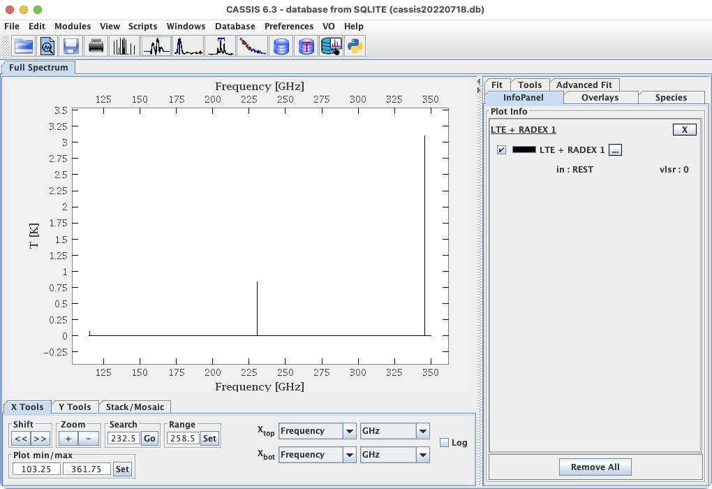
Finally, to display the modeled spectrum, click on the
Display button. Note that you will get a warning due to the large number of points;
however, since there are few CO lines in the selected range, the computation will nonetheless be very fast.
For the parameters in the above figure,
you will obtain the following: