


Common functionalities
| Contents |
Interactive graphical tools
Many tools can be used to interactively examine a spectrum plotted via one of the modules described in Section 2:
- With the mouse:
- Zooming in is performed by selecting the region with a left-click on your mouse from the upper-left corner to the lower-right corner of the region of interest.
- Zooming out is done by holding a left-click while going from the lower-right to the upper left of the display window.
- The cursor gives the coordinates (x-axis, y-axis) when pressing the "Shift" button while moving the mouse over the plot.
- Left clicking on the spectrum will give the name and some parameters of the closest transition in a small pop-up window (except for an observational datafile without any overlays).
- Right-clicking on the spectrum allows to manage the plot via the usual java "Properties..." panel.
- File > Save (top menu) will allow you to save the spectrum in different formats such as pdf, png, votable.
- Via the X Tools and Y Tools tabs at the bottom of the window:
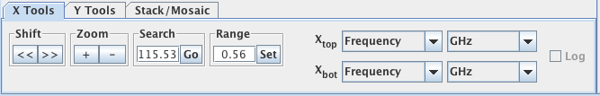
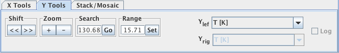
- Shift: to displace the plotted spectrum by half of the width of the window, toward increasing (>>) or decreasing (<<) values of the axis.
- Zoom: to zoom in (+) or out (-) by a factor of 2.
- Search: typing a value in the box and hitting the carriage return key or clicking on "Go" will center the axis on that value.
- Range: typing a value in the box and hitting the carriage return key or clicking on "Set" will modify the plotted range to match the specified value.
- Xbot / Xtop : allows you to toggle the X-axis between different scales (frequency, velocity, wavelength, wavenumber, energy) and different associated units.
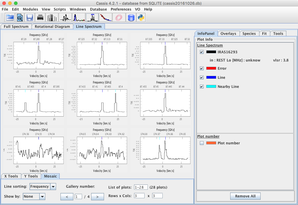
- The Stack/Mosaic tab is useful in the "Line Spectrum" (top) tab only:
- In the Mosaic tab (first available after clicking "Display" in the "Line Analysis" window),
List of plots allows you to specify a subset of lines, e.g., 1,3-5,8 ;
the arrows (< and >) under
Gallery number allow you to flip through all the pages needed to account for the lines specified in the "List of plots" field (default: all the lines found by the "Line Analysis" window).
- In the Stack tab (available after double-clicking on a chosen line from the mosaic),
the arrows (< and >) next to
Plot number allow you to flip through all the lines found
by the "Line Analysis" window.
The green bended arrow above the "Stack" tab allows you to go back to the mosaic.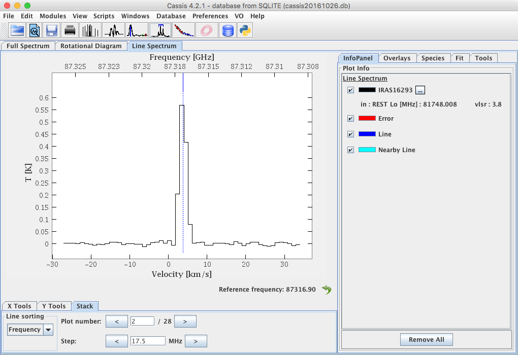
- In both "Stack" and "Mosaic" tabs, you can choose line sorting by frequency, Eup or Aij.
- In the Mosaic tab (first available after clicking "Display" in the "Line Analysis" window),
List of plots allows you to specify a subset of lines, e.g., 1,3-5,8 ;
the arrows (< and >) under
Gallery number allow you to flip through all the pages needed to account for the lines specified in the "List of plots" field (default: all the lines found by the "Line Analysis" window).
- The plot panel in which the spectrum is displayed is divided in 3 regions:
- top: line information (in "Line Analysis") or line lists (in "Spectrum Analysis")
- middle: spectrum and/or model
- bottom: other species
Note that in several places in CASSIS, you will encounter greyed out buttons/fields. This means that we are planning on having these functionalities in future versions of CASSIS, but that they are not yet available.
Inspect and analyze the spectrum (right-hand side tabs)
In the "Full Spectrum", "Loomis Spectrum" and "Line Spectrum" (top-left) tabs, the plot can be managed using the tabs on the right-hand side of the window:
- InfoPanel shows all the data currently in memory.
- Checking/unchecking the box on the left of a dataset will display/remove the corresponding spectrum.
- Clicking on the 'X' on the right of a dataset will remove it from memory.
- Clicking on the color box of a given dataset will bring a pop-up window allowing you to change the color and other plot parameters.
- Overlays gives the possibility to overlay other data files and linelists.
- Species gives the possibility to overlay the positions of the transitions of all the species in the selected template, which are present in the displayed range. This overlay can be customized by specifying the following parameters: Thresholds and Settings (Eup, Aij), Template (choose from the pull-down menu).
- Fit tab allows baseline and line fitting with
two different algorithms: Amoeba fitter
and Levenberg-Marquardt fitter.
- Manage Components pull-down menu:
allows to add as many components as desired, one at a time.
The component can be either a baseline (polynomial or sinusoidal)
or a line (Gaussian, Lorentzian, Voigt, or Sinc) ;
mathematical definitions are given in this
pdf file.
The following user cases are described step-by-step in the linked pdf files :- fitting a simple (polynomial) baseline in Spectrum Analysis
- fitting a single Gaussian in Spectrum Analysis
- fitting multiple Gaussians in Spectrum Analysis
- click on "Manage Components", select "Add Line" -> "Gaussian" ;
the parameters appear with blue fields for the initial guesses
(which CASSIS automatically fills in with the next step).
Grey fields are non editable and will show the statistical errors once the fit is done.
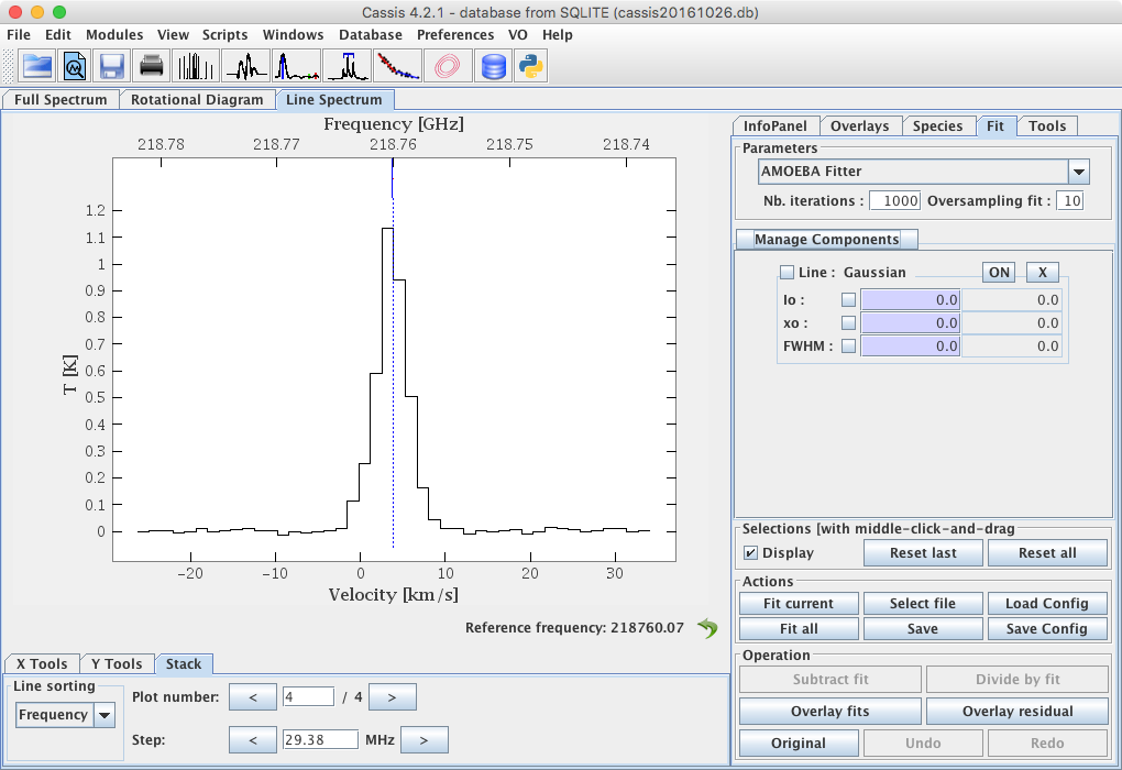
- select the domain to be fitted by clicking-and-dragging the middle mouse button over the region.
If you do not have an external mouse,
the middle mouse can be emulated with "Alt"+click on a Mac or "Ctrl"+click on a PC.
Note the number displayed on the plot (here in K.km/s): it is the value of the first moment under the blue area.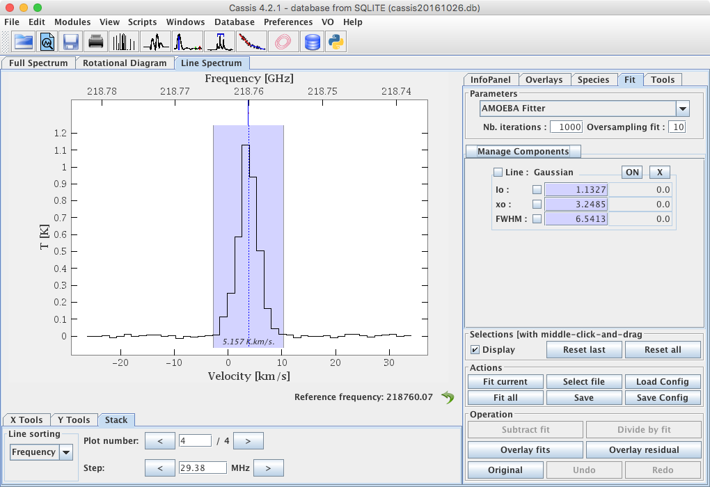
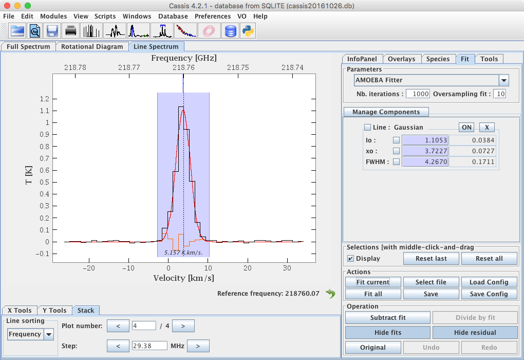
- click on "Fit current" ; the fit is in red, the residuals are in orange.
- Actions panel:
- Fit current: fits the last component added.
- Fit all: fits all the lines simultaneously (only in the "Line Spectrum" tab) ; CASSIS will ask the user to open an existing file or create a new one in which the results of the fits will be saved.
- Select file: opens a pop-up window to select an existing file (to append fit parameters) or to create a new one.
- Save: save the parameters of the current fit in the file opened with "Select file".
- # : value corresponding to the order in which the component was added in the "Manage Components" panel.
- Transition : name and quantum numbers of the transition from the database
- Frequency(Mhz) : frequency in MHz from the database
- Eup(K) : energy of the upper level in K from the database
- Aij : Einstein A-coefficient (in s-1) from the database
- FitFreq.(xunit) : fitted frequency
- deltaFitFreq. : associated 1-sigma error
- Vo(km/s) : fitted velocity in km/s
- deltaVo : associated 1-sigma error
- FWHM_G(km/s) : fitted FWHM for a Gaussian component
- deltaFWHM_G : associated 1-sigma error
- FWHM_L(km/s) : fitted FWHM for a Lorentzian component
- deltaFWHM_L : associated 1-sigma error
- Int(yunit) : fitted intensity at line center
- deltaInt : associated 1-sigma error
- FitFlux(yunit.km/s) : fitted flux in K.km/s
- deltaFitFlux : associated 1-sigma error
- Freq.I_Max(xunit) : frequency at the observed maximum intensity
- V.I_Max(km/s) : velocity at the observed maximum intensity
- FWHM(km/s) : parameter equal to Flux/I_Max and representing roughly the "observed" FWHM
- I_Max(yunit) : observed maximum intensity
- Flux(yunit.km/s) : integrated intensity (1st moment) in the region selected with the mouse
- deltaFlux :
- RMS(unit) : observed rms in unit=mK if spectrum is in K, and unit=yunit otherwise ; this parameter is non-zero and relevant only if a baseline was fitted (and subtracted) prior to fitting the line component
- deltaV(km/s) : channel spacing in velocity scale
- Cal(%) : calibration uncertainty in % ; this parameter is highly dependent on observing conditions and has been set to 0.0 by default : the user should edit the fit file to replace the zeros by the desired values
- Telescope : path to the telescope file
- Selections and Operation panels: all toggle buttons should be self-explanatory. Some of them are not yet active but will be in a forthcoming version of CASSIS. Moreover, depending on current action in the fitting process, the appearance of the toggle button is not always updated. We are working on solving this issue.
- Manage Components pull-down menu:
allows to add as many components as desired, one at a time.
The component can be either a baseline (polynomial or sinusoidal)
or a line (Gaussian, Lorentzian, Voigt, or Sinc) ;
mathematical definitions are given in this
pdf file.
- Tools tab allows you to perform mathematical operations on spectra:
- subtract or add two spectra,
- add a constant to a spectrum,
- multiply a spectrum by a constant,
- apply smooth Hanning,
- average spectra,
- resample,
- change from Ta to Tmb, or the opposite,
- change the frequency frame (different Vlsr),
- change from REST to SKY frequency, or the opposite,
- change from air to vacuum wavelength or the opposite,
- apply redshift correction.
- Advanced fit tab allows you to perform constrained fits : see section 3.3
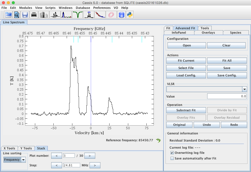
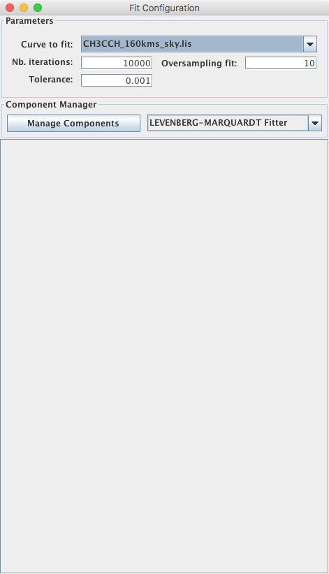
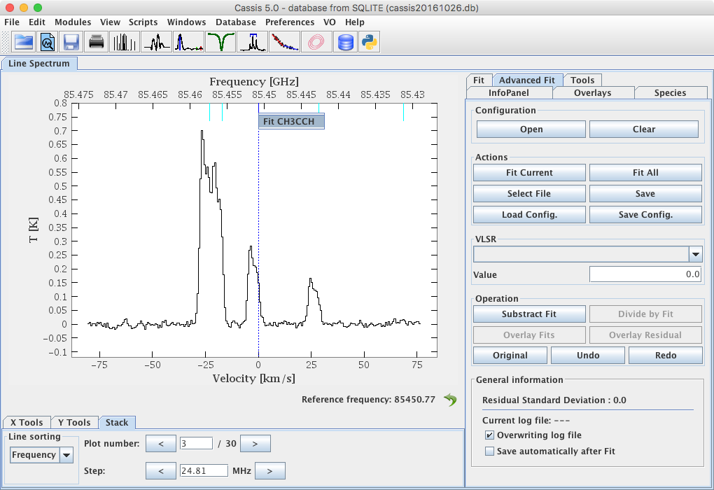
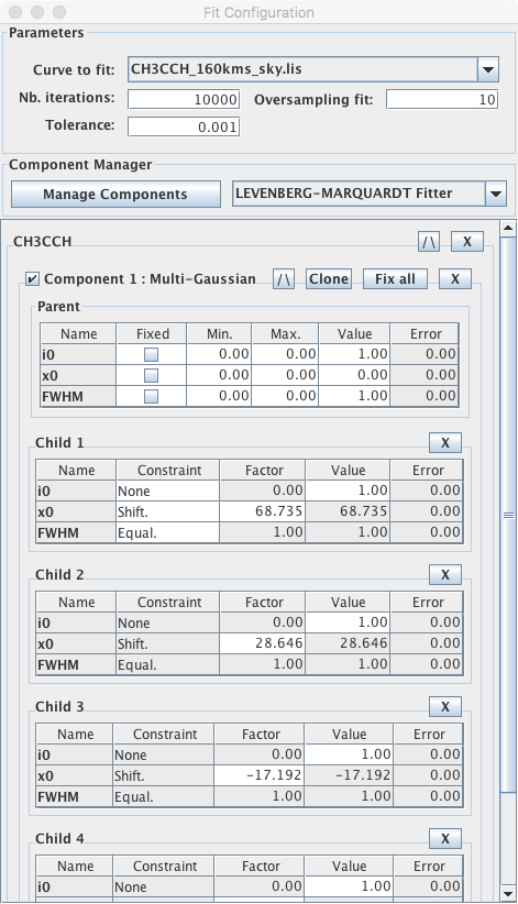
Advanced fit (right-hand side tabs)
The advanced fit allows you to perform fits on multiple transitions simultaneously, using constraints on the parameters. One of the great advantages is that CASSIS can automatically provide you with the number of line components corresponding to the number of transitions found in the database, and for each line component, CASSIS fills in the velocity/frequency offsets based on the information found in the database.Have a look below at the video for an example, and at the screenshots for an illustration of the advanced fit interface.
 |
 |
 |
 |