(Last update : 07/28/17)

• 1 About CASSIS
  1. 1.1 How the document is organized
  2. 1.2 Starting CASSIS and displaying a spectrum
  3. 1.3 Snapshots
  4. 1.4 Copyright Notice

• 2 Modules
  1. 2.1 Spectrum Manager and ASCII parser
  2. 2.2 Spectrum Analysis
  3. 2.3 LTE+RADEX
  4. 2.4 Loomis Wood
  5. 2.5 Line Analysis
  6. 2.6 Rotational diagram
  7. 2.7 χ² Plot

• 3 Common functionalities
  1. 3.1 Interactive graphical tools
  2. 3.2 Inspect and analyze the spectrum (right-hand side tabs)
  3. 3.3 Advanced fit (right-hand side tabs)

• 4 Databases
  1. 4.1 Configuration
  2. 4.2 Templates
  3. 4.3 Database Creation

• 5 Interoperability
  1. 5.1 SAMP
  2. 5.2 SSAP

• 6 Scripts

• 7 Caveats and tricks

• 8 CASSIS in HIPE

• 9 Video tutorials

Rotational diagram

---

Contents Utility of the Rotational diagram How does it work?

Utility of the Rotational diagram

The Rotational Diagram tool can be used to plot y=ln(Nu/gu) as a function of x=Eup/k. Values for the y-axis depend on the user's choice (see this section) and are extracted from the data file containing the fit (and other) parameters saved during a Line Analysis session ; the method to create such a file containing the necessary information for the computation of the uncertainties is described in the first part of this section.
Note that it is important to have selected the appropriate Telescope in your Line Analysis, even if you do not perform Tmb -> Ta conversion at this stage. If you did not choose the correct Telescope, just edit the file containing the fits from the Line Analysis and change the Telescope name by the appropriate one for each line before running the Rotational Diagram.

How does it work?

The first thing to do is to produce a .rotd (.txt for CASSIS versions prior to 3.8) datafile containing, for each transitions:

• the spectroscopic parameters
• the integrated intensity from the line fit (Gaussian, Lorentzian or Voigt profile ; in each case, the first moment is always computed by CASSIS) ; note that, currently, the rotational diagram analysis only works with integrated intensities in K.km/s
• the rms and calibration uncertainty (necessary for the overall uncertainty computation)
• the telescope name

To create such a file, perform the following steps:

1. Open the CASSIS Line Analysis module, load your data file, select a species, set your thresholds and click "Display"
2. Select the first transition (double-click), open the "Fit" panel, click on "Manage Component" -> "Add baseline" and choose the desired type of baseline ; adjust the parameters (e.g., the order of the polynomial), and select line-free region(s) on the spectrum with a middle-click-and-drag ;
   Then click on "Fit all" and "Create a new File" in the pop-up window.
3. Check that all your transitions are fitted correctly in the mosaic panel (click on the icon ).
4. If some baselines are wrong (presence of alien lines for example), click on this/these particular window(s), select a new region to fit the baseline and click on "Fit current".
5. If necessary, within the mosaic panel do a "Subtract Fit". The baseline will be therefore removed for all the windows.
6. To fit all the transitions with a Gaussian Fit for example: select the first transition, remove the Baseline component (by clicking on "X" or "ON" to disable) and click on "Reset all" to remove all selections.
   Click on "Manage Component" -> "Add Line" -> "Gaussian", select the window where you want to perform the fit (large enough for the other transitions that you cannot see right now). Finally, click on "Fit all" (in the pop-up window, Open the existing .txt file you created in step 2). Check that you agree with the line fitting for all the transitions (mosaic panel). If not, re-do the line fitting for the transition(s) you want, using the "Fit current" button.
7. Open the .txt file in an editor (or better in a spreadsheet) and enter the instrument calibration error for each transition in the column before last.
8. Your file is now ready to be opened in the Rotational Diagram module. When you do so (see below), the error bars displayed on the figure take into account the rms and the calibration uncertainty, necessary to compute the uncertainty on the integrated intensity (see the document "Formalism for the CASSIS software").
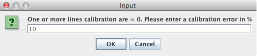
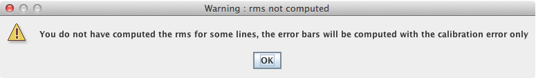
   If cal=0, then CASSIS asks you the value you want to implement (the same value will be set for all lines) ; if rms=0, you get a warning (see below)

Click on the third menu, Modules, and choose Rotational Diagram. Alternatively, click on the icon . In both cases, a Rotational Diagram window opens:

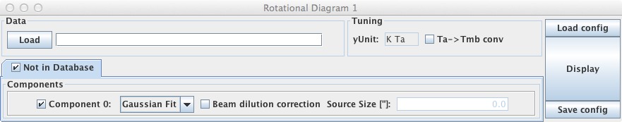
Click on the 'Load' button : this opens a file browser that allows you to select the file you created with the above steps.
If cal=0 in the datafile, a window opens asking you the value you want to implement (the same value will be set for all lines) :

If rms=0 in the datafile, you get the following warning :

Choose the type of integrated intensity you want to use to calculate ln(Nu/gu) : Gaussian fit or 1st moment. If you need to correct for beam dilution (as in the figure below) and/or to convert the temperature scale, check the appropriate box(es). In case of beam dilution correction, you will need to specify the appropriate source size in arcseconds.

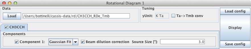
Finally, click on 'Display' to plot the points:

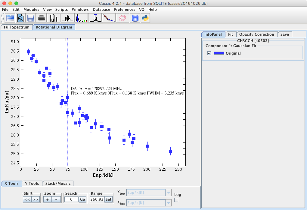
You can display relevant information contained in the datafile by clicking on any point as in the above figure. Note that the format of the input datafile has evolved, so that the amount of information displayed depends on what is in the datafile. The latest version of CASSIS can read input files created by any older version.

Specific tabs:

• Fit:
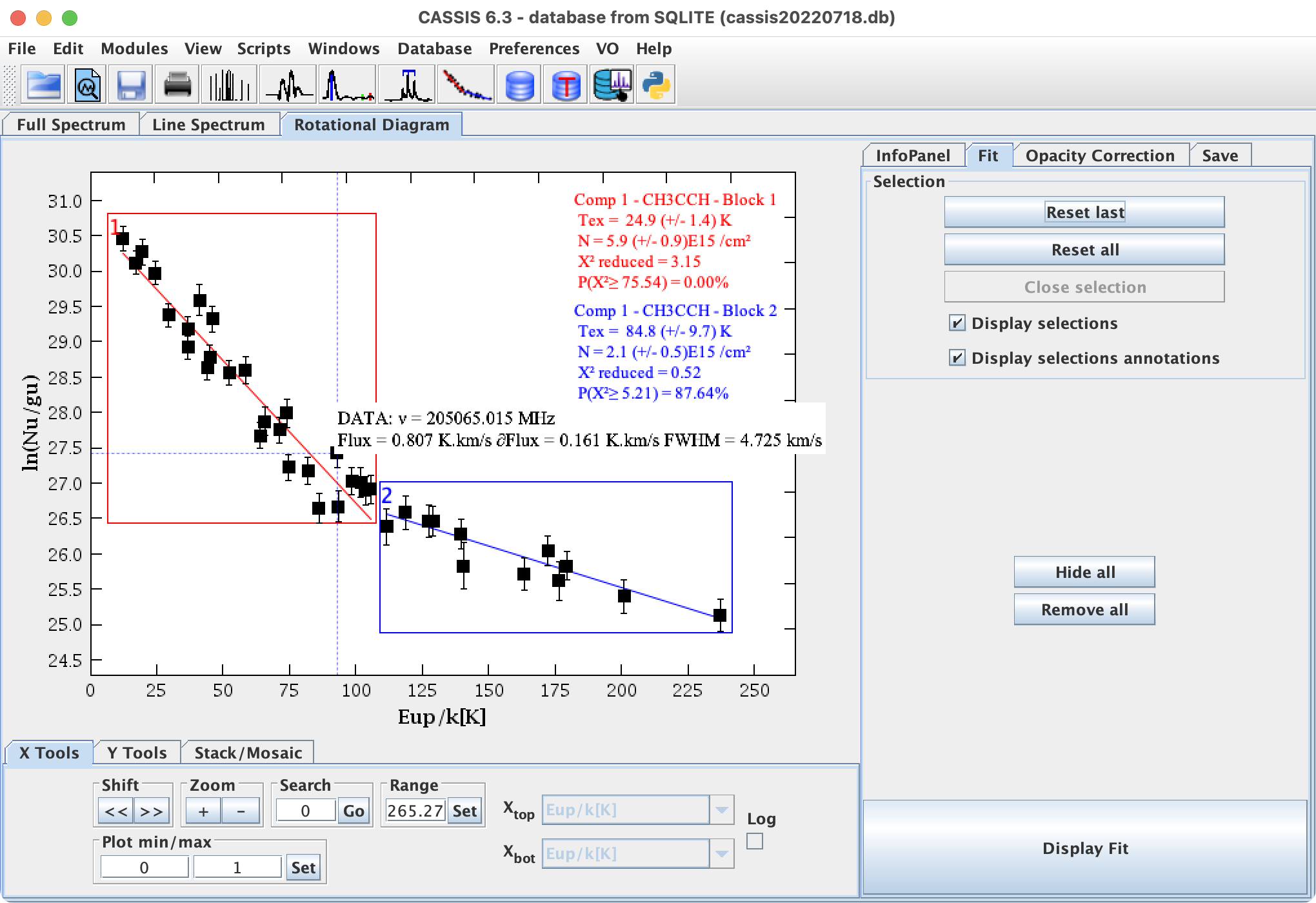
  • To perform a linear fit to all the points, simply click the 'Display Fit' button
  • To perform the fit to a subset of points, use the middle button of your mouse (or 'alt'+click if you do not have access to an external mouse) to select the chosen points. This action opens a selection session and the 'Close selection' button becomes available. You can choose to close the selection after choosing a single group of points or you can 'build' a subset of points by choosing one or a group of points anywhere on the plot; you can de-select the last point(s) with 'Reset last selection'. when you are satisfied with your selection, click on 'Close selection'. Repeat selection sessions as necessary. The selections appear in different colors and are numbered. For clarity, it is advised to perform a small number of selections.
    Finally, click on 'Display Fit'. The fits corresponding to the different selections will appear in different colors:
  
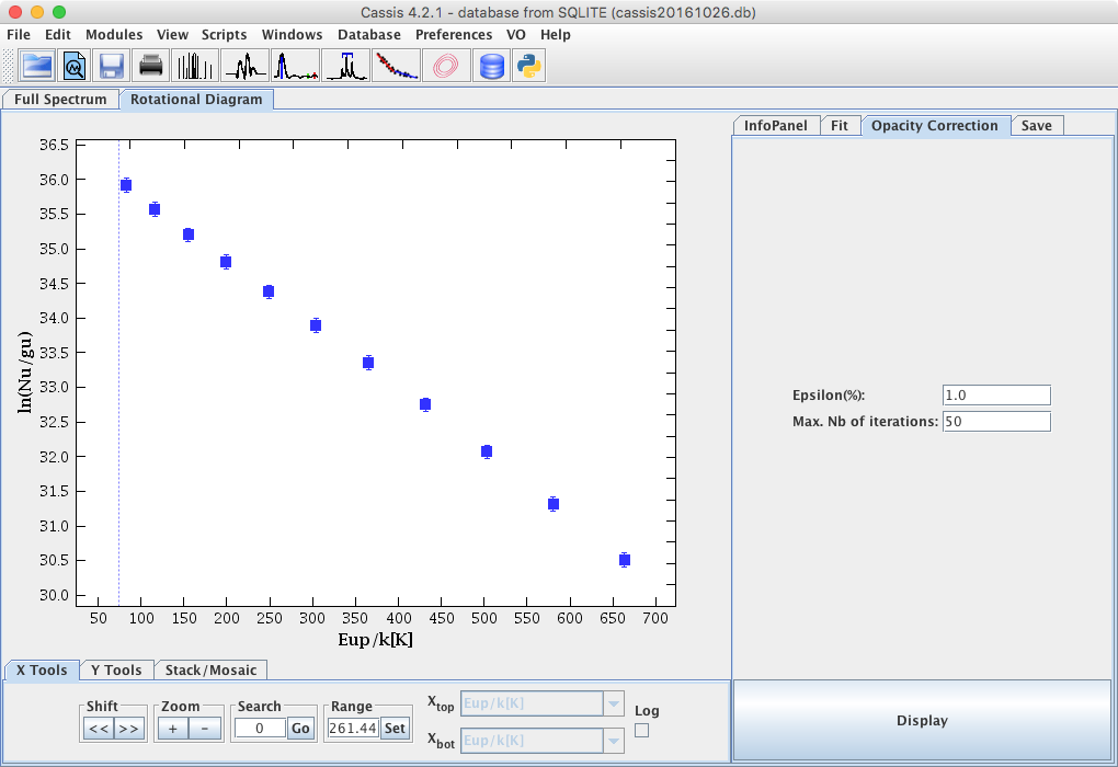
• Opacity correction: CASSIS can perform opacity correction on lines which are not blended and not part of a multiplet. This correction is an iterative process (see the document "Formalism for the CASSIS software") which stops when the difference between the last two iterations is smaller than the specified value ("epsilon", in %), or when the specified number of iterations has been reached, whichever comes first.
  
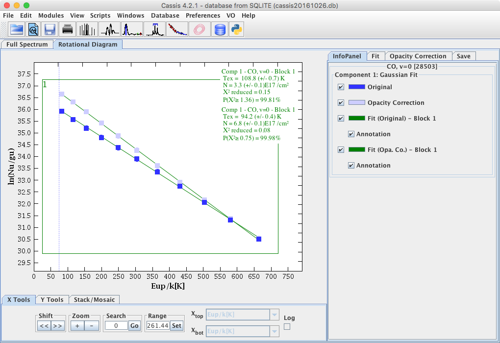
  Clicking on 'Display'and going to the InfoPanel tab yields:
  
  Notes:
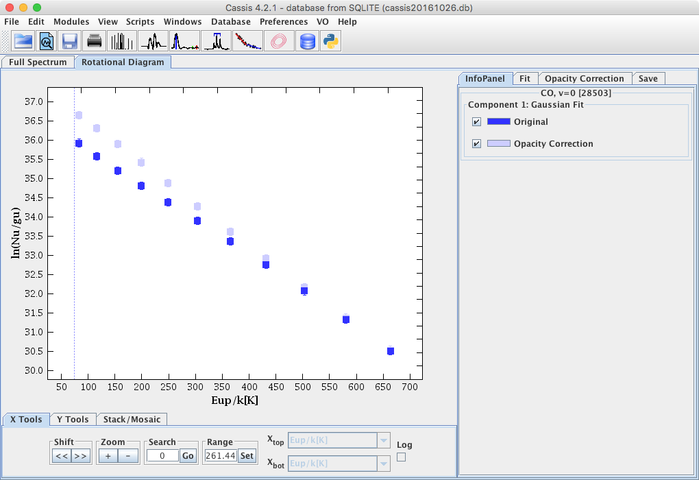
  • If a fit is performed on opacity corrected data, CASSIS will do it on both the original and corrected data; both fits will have the same color since color assignment for the fits is done per block (this can easily be changed by clicking on the color in the InfoPanel tab).
    
  • This correction works best on mildly optically thick data.
• Save: to save the displayed values in an ASCII file.

---