(Last update : 07/28/17)

• 1 About CASSIS
  1. 1.1 How the document is organized
  2. 1.2 Starting CASSIS and displaying a spectrum
  3. 1.3 Snapshots
  4. 1.4 Copyright Notice

• 2 Modules
  1. 2.1 Spectrum Manager and ASCII parser
  2. 2.2 Spectrum Analysis
  3. 2.3 LTE+RADEX
  4. 2.4 Loomis Wood
  5. 2.5 Line Analysis
  6. 2.6 Rotational diagram
  7. 2.7 χ² Plot

• 3 Common functionalities
  1. 3.1 Interactive graphical tools
  2. 3.2 Inspect and analyze the spectrum (right-hand side tabs)
  3. 3.3 Advanced fit (right-hand side tabs)

• 4 Databases
  1. 4.1 Configuration
  2. 4.2 Templates
  3. 4.3 Database Creation

• 5 Interoperability
  1. 5.1 SAMP
  2. 5.2 SSAP

• 6 Scripts

• 7 Caveats and tricks

• 8 CASSIS in HIPE

• 9 Video tutorials

Line Analysis

---

Contents Utility of the Line Analysis tool How does it work?

Utility of the Line Analysis tool

The Line Analysis tool can be used to look into class formatted files (.30m, .bur, etc....) or fits files in order to search for identified species. The headers are read and the spectrum is displayed in the graphical interface. Also, all the species present in the databases can be displayed accordingly as tick marks and consequently show the location of those potential species in the spectrum. Lines in the spectrum can therefore be identified easily. Also this tool can be used to fit a baseline and remove (or divide) it from the the spectrum.

How does it work?

Click on the third menu, Modules, and choose Line Analysis. Alternatively, click on the icon . In both cases, a pop-up window opens:

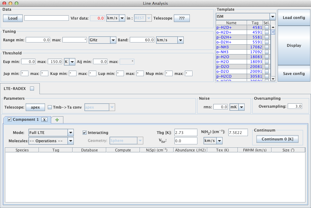
You first need to select a datafile by clicking the Load button. This datafile must be an observation file (.bur, .class, .30m, etc...) that can contain many different scans. Those files need to contain the header with the LO frequency and the telescope IF frequency. You can select the tuning range, and a Threshold to limit the data you want.

You then need to select one single species within the Template section. The template is chosen in the drop-down menu. You can search a species using its formula by right-clicking on "Name". WARNING: the name of a given species can be different in different databases, e.g. NNH+ or N2H+.

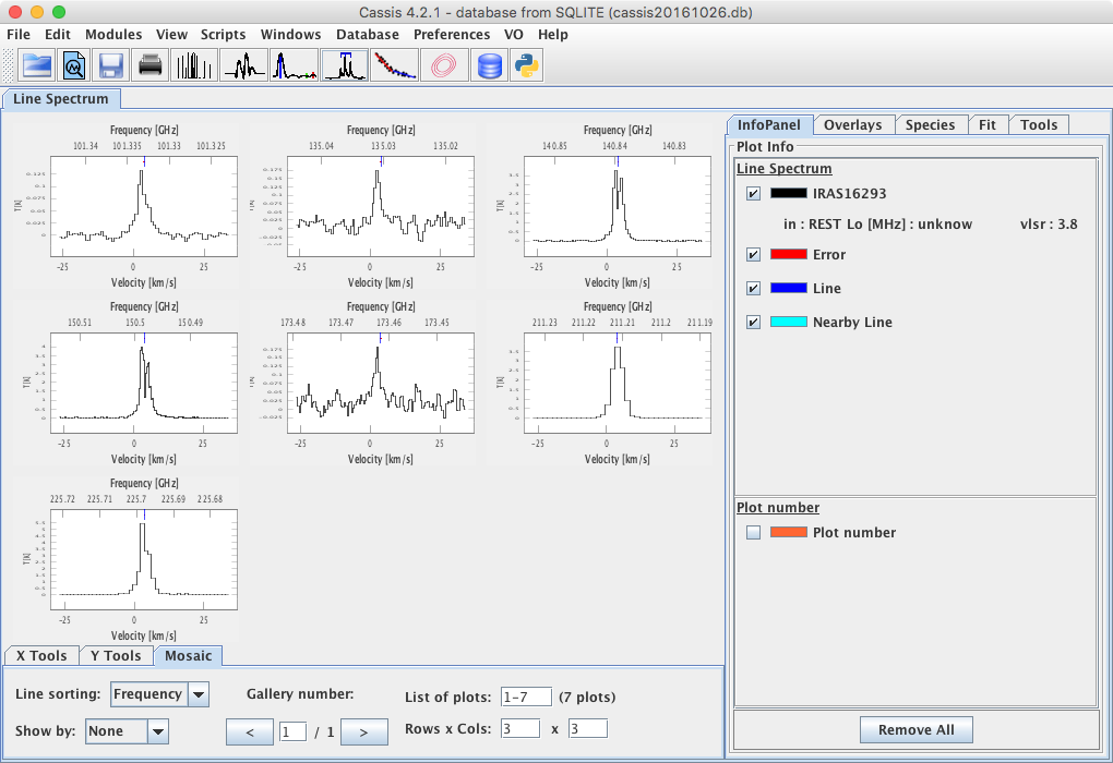
When you click on the Display button, CASSIS will find and display all the lines in your datafile that match the tuning range and thresholds. The lines are displayed in a mosaic of panels, each panel having a bandwidth equal to Band.
A graphic window similar to the one below will appear as a result of the Display.

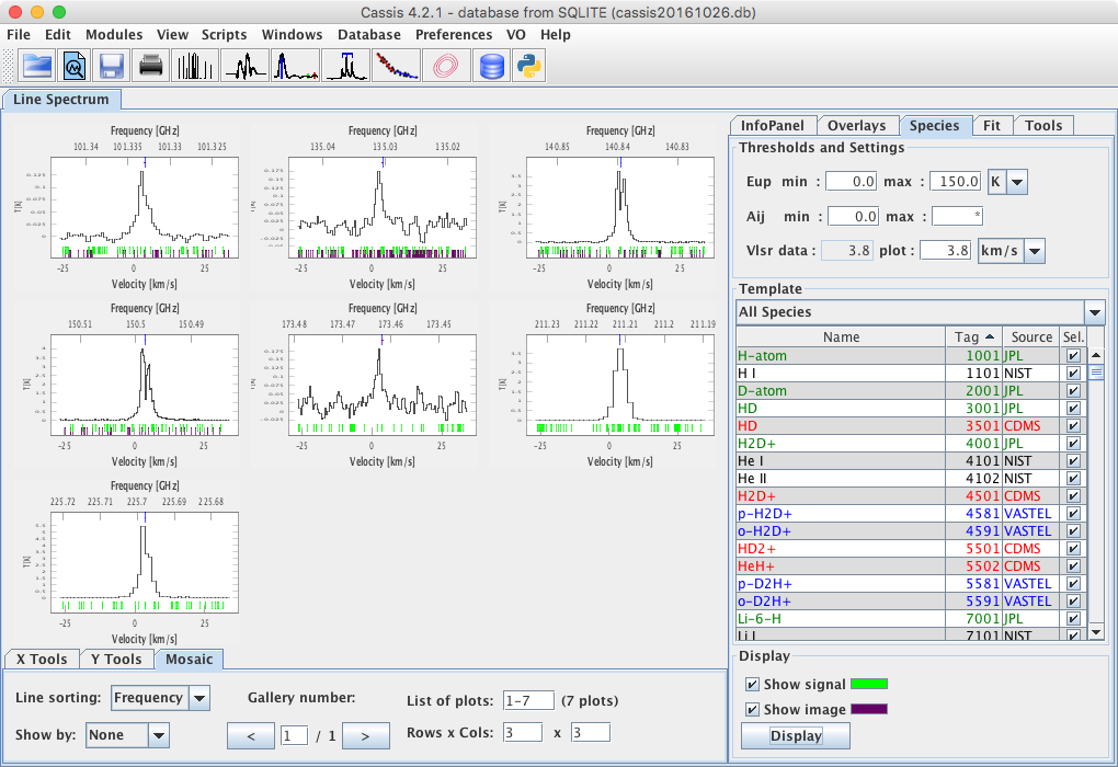
If you want to view all the species potentially present in the spectra, click on the Species tab, select the desired template (in the figure below, we selected "All Species" and ordered them by tag by a click on the "Tag" column header), set the chosen thresholds and settings and click display. CASSIS will show the transitions found in the database that are present in the signal and image (if it applies) bands, as in the figure below.

If you want to overlay a model, check the LTE-RADEX box in the "Line Analysis" window. You may vary the column density, excitation (or kinetic) temperature, etc ... of the species you selected (see the LTE+RADEX module for more details), and click on the Display button.
If you display the other species from the "Species" tab and double-click on one of the panels, the graphic window will then be similar to the figure below.

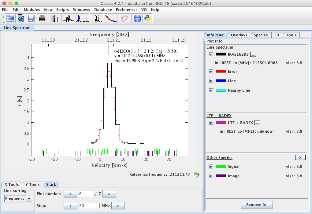
At the bottom you can see the Plot number of the lines that have been found for your species. On this plot, 7 lines of o-H2CO have been found and are plotted in back. In the Info Panel the informations concerning the plot are displayed:

1. black: your data file,
2. magenta: the LTE or RADEX model you selected above,
3. red: the potential error associated with the observation file,
4. blue: the location (in frequency) of the selected line,
5. turquoise: the location (in frequency) of any nearby line of the selected species,
6. green: the location (in frequency) of any other species in the signal band,
7. purple: the location (in frequency) of any other species in the image band.

Note that you can change the color by clicking of the color boxes.
This Line Analysis tool can also be used to fit a baseline as well as line profiles as indicated as in this section.

---