(Last update : 01-Jul-24)

• 1 About CASSIS
  1. 1.1 How the document is organized
  2. 1.2 Starting CASSIS and displaying a spectrum
  3. 1.3 Snapshots
  4. 1.4 Copyright Notice

• 2 Modules
  1. 2.1 Spectrum Manager and ASCII parser
  2. 2.2 Spectrum Analysis
  3. 2.3 LTE+RADEX
  4. 2.4 Loomis Wood
  5. 2.5 Line Analysis
  6. 2.6 Rotational diagram

• 3 Common functionalities
  1. 3.1 Interactive graphical tools
  2. 3.2 Inspect and analyze the spectrum (right-hand side tabs)
  3. 3.3 Advanced fit (right-hand side tabs)

• 4 Databases
  1. 4.1 Configuration
  2. 4.2 Templates
  3. 4.3 Database Creation

• 5 Interoperability
  1. 5.1 SAMP
  2. 5.2 SSAP

• 6 Scripts

• 7 Caveats and tricks

• 8 Video tutorials

Loomis Wood Analysis

---

Contents Utility of the Loomis Wood Analysis tool How does it work?

Utility of the Loomis Wood Analysis tool

A Loomis-Wood diagram is a two-dimensional peak diagram in which:

• the occurrence of a transition is plotted versus frequency/wavenumber/wavelength, in segments of a given width.
• the height of a line is proportional to the column density, weighted by the partition function at the chosen excitation temperature.

Interactive Loomis-Wood assignment programs help assign spectra, and estimate column densities.
Note that, at the moment, for the calculation of the line intensity (and hence the estimate of the column density) to be correct, the data must be in Jy. Any other unit will only allow you to determine relative column densities (assuming you look at more than one species).

How does it work?

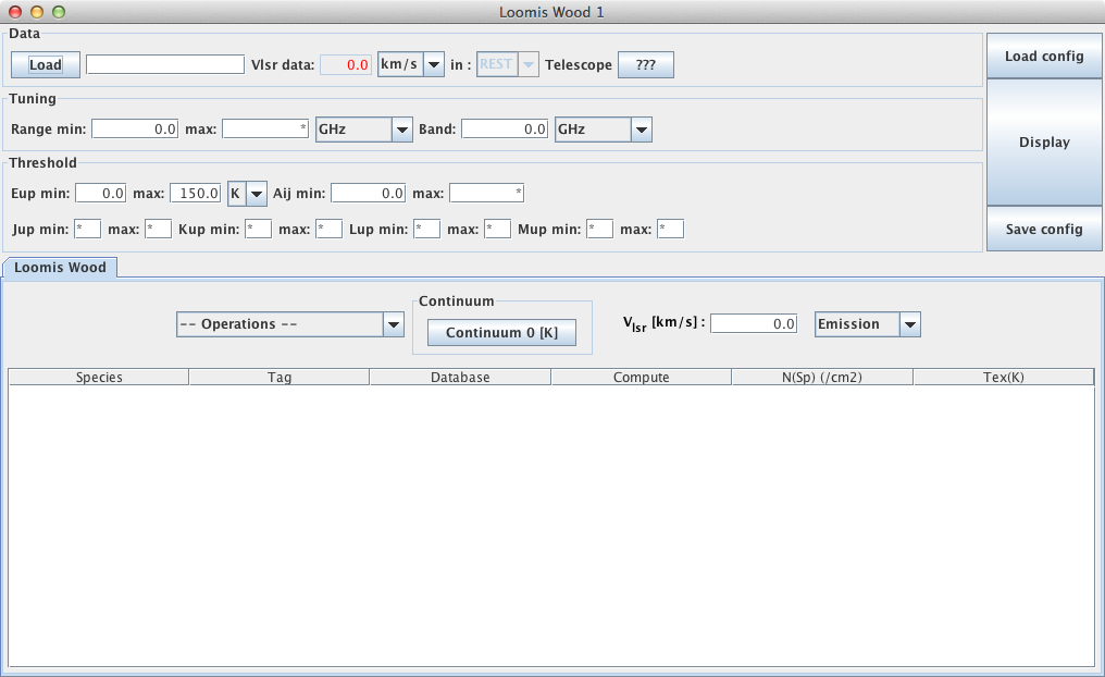
Click on the menu Modules, and choose Loomis Wood. Alternatively, click on the icon . In both cases, a pop-up window opens:

Select an observational datafile by clicking the Load button. You can change the constraints on the data that will be displayed by modifying the fields in the Tuning and Threshold sections. An important parameter here is Band: its value should be equal to the separation between the transitions of the species of interest. For example, for ¹²CO, 115 GHz or 3.835 cm^-1.
In the Loomis Wood tab, select your template/species, choose a continuum file if desired, V_lsr, and whether the line is expected in emission or absorption.

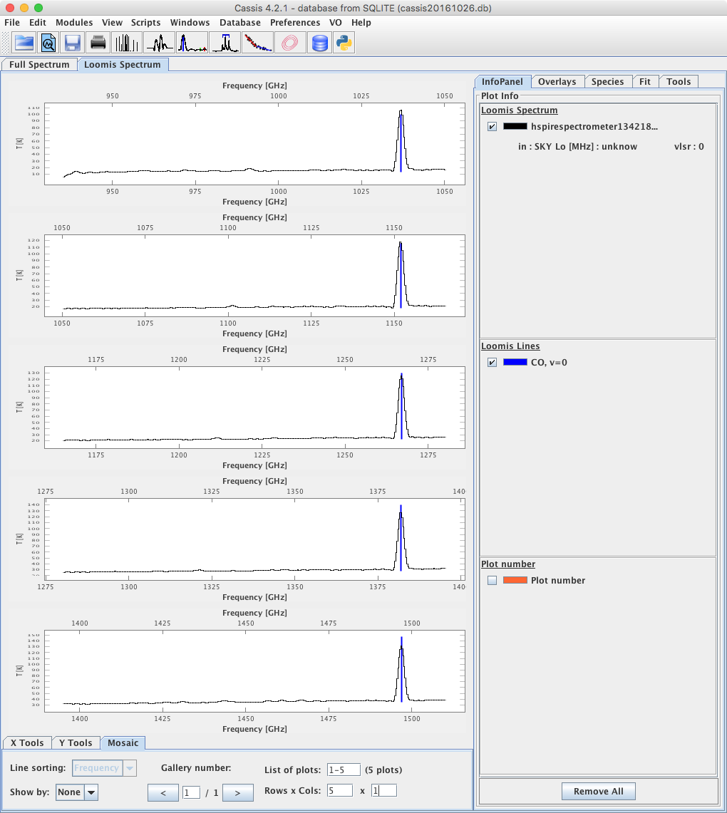
When you click on the Display button, CASSIS will find and display all the lines in your datafile that match the tuning range and thresholds. The lines are displayed in a mosaic of panels, each panel having a bandwidth equal to Band. When the bandwidth is equal to the separation between the transitions of, e.g., CO, then a Loomis-Wood diagram with aligned CO transitions is obtained.
A graphic window similar to the one below will appear as a result of the Display.

---